As Machine Learning (ML) and Deep Learning (DL) techniques become more sophisticated, they are being applied to an increasing number of tasks. One such application is the search for exoplanets, which we will discuss in this blog post. We’ll focus on the Transit Method and what role Machine Learning can play in successfully overcoming the pertaining challenges.
INTRODUCTION
Machine and Deep Learning techniques are here to stay. Their automated nature and their learning ability offer the possibility of managing any type of data. Its wide variety of techniques supports a multitude of disciplines, including astrophysics and, in particular, the search for exoplanets, with special relevance in the so-called transit method.
EXOPLANETS AND THE TRANSIT METHOD
An exoplanet is a planet that orbits a star outside of our solar system. Most exoplanets are found using the Radial Velocity Method, which detects the tiny wobbles of a star caused by the gravitational tug of an exoplanet orbiting it. Other methods of exoplanet detection include Transit Photometry, which looks for the slight dip in a star’s brightness that occurs when an exoplanet passes in front of it, and Direct Imaging, which captures images of exoplanets directly.
In this article, I’ll focus on the Transit Method in which “ an exoplanet blocks light reaching the Earth from the star it orbits”. Unsurprisingly, detecting one is an extremely complicated task.
The search for exoplanets has its main detection site in outer space, outside the influence of our beloved atmosphere, for the simple fact that most of the light we receive from space is absorbed by it. That’s why telescopes have been instrumental in the search. First COROT, then Kepler/K2, and lately TESS, telescopes expanded our knowledge of the great variety of exoplanets we are surrounded by. As of August 23, 2022, the NASA Exoplanet Archive has confirmed the existence of 5071 exoplanets with more than 7000 other possible candidates.
One of the most daunting aspects of starting my Ph.D. was the immense amount of data processing that had to be done. The Kepler space telescope had recently finished its main mission and NASA had even been able to recover it from a double failure in its pointing system to continue operating with the renamed K2 mission.
THE TWO CHALLENGES: TOO MANY LIGHT CURVES AND TOO MUCH NOISE
To illustrate the dimension of the problem in the search for exoplanets, Kepler yielded some 150,000 light curves in its first mission and some 40,000 light curves per quarter in its almost six years operating the K2 mission. (A light curve is a graph of light intensity of a celestial object or region as a function of time.)
In other words, from the Kepler mission alone, we have more than a million light curves to analyze and classify. The TESS mission yielded millions of light curves. These are some of the greatest problems the field faces today:
- An abundance of data to analyze, which for an expert or even a small group of experts would take years of work and would almost certainly lead to errors in the analysis and classification.
- The choice of a suitable aperture for each star to reduce signal contamination from nearby stars as much as possible.
Let’s revisit the definition of the light curve,simplest and most practical being: “the amount of measured light that reaches the Earth per unit of collecting area (diameter of our telescope) and per unit of observation time”. This form of observation is what astronomers call “Photometry” and, typically, a Kepler light curve has the shape shown in Figure 1.
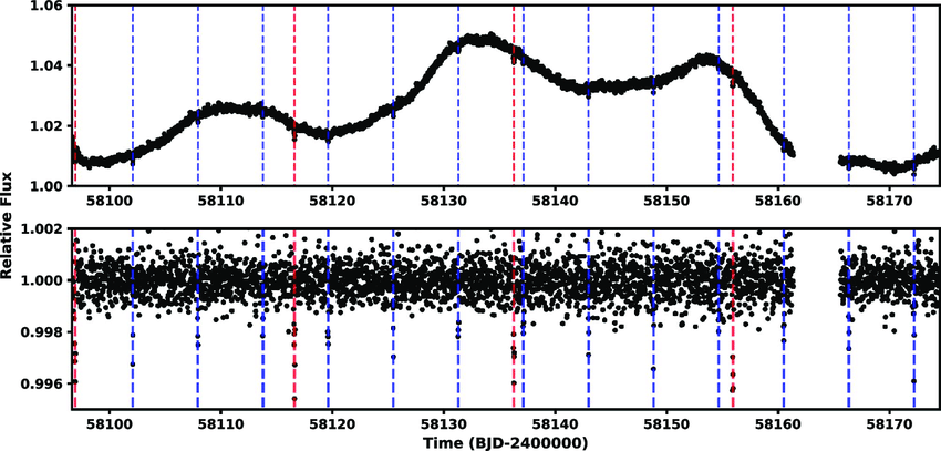
Figure 1: Light curve of K2-264 obtained with the Kepler space telescope. The planetary system of two transiting planets. The vertical red and blue lines indicate their position. The upper image corresponds to the light curve before flattening, and the lower image corresponds to the light curve after flattening.
But to understand this definition and its application to the field of astrophysics, it is best to answer the following questions: How is a light curve obtained and what is an exoplanetary transit?
To understand this, we need to take a closer look at our solar system. By now, everybody knows the dynamics behind a solar eclipse, which, in essence, is the blocking of the light of our star, the Sun, by the Moon, our satellite (see figure 2).
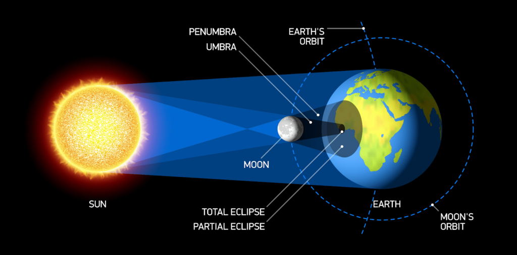
Figure 2: Diagram of a solar eclipse.
Transit is what occurs when Mercury, the closest planet to the Sun, blocks a tiny fraction of the Sun’s light when interposed between the Sun and the imaginary line that joins the Earth and the Sun (line of sight). Normally this phenomenon is not visible to the naked eye and we need a telescope to see it in detail (figure 3).
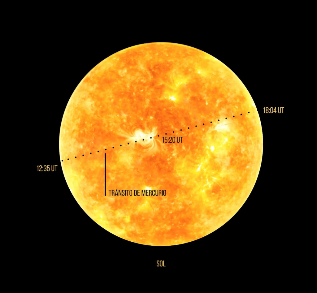
Figure 3: Image of the Sun and representation of the transit of Mercury at different times from November 11, 2019.
Imagine that I am a great amateur photographer and adapt my camera to a telescope to take pictures of the Sun during Mercury’s transit. In the morning, I take a picture (time unit, t), and by adding up all the pixels of the camera where the Sun is, I obtain a number of counts (photons) that I will transform into a number of measurable physical quantities. Let’s call these quantities “Luminosity” (L). Obtained a point (t, L), then, I take another and another, and so on in a regular way until the night arrives. If I now make the typical Cartesian graphical representation of the school assuming the “x” axis as the time axis and the “y” axis as the Sun’s luminosity, we would see something very similar to what the following video depicts.
Now that we are clear about what a light curve is, let’s apply the same reasoning to other stars. Since the luminosity is much smaller, observing transits of other planets from the surface of the Earth is very difficult and we have to go to space to get them. A difference between the transit of Mercury and that of an exoplanet observed from space is how we take the pictures, which, typically, for the Kepler/K2 space mission is three seconds taken over three months. This is what we observe in Figure 1.
KEPLER AND TESS: TWO WAYS, ONE GOAL
It is important to differentiate between the pictures taken by Kepler/K2 and the pictures taken by TESS because they are different solutions. The technical limitation of the Kepler mission meant that it transmitted to Earth only small cuttings of a few pixels from each of the 84 CCDs (Charge Couple Devices) of which it was composed. The CCD pixels work similarly to those in a flat-panel television: but instead of emitting light, they collect light, or rather electrons. These pixel cutouts are shown in Figure 4.
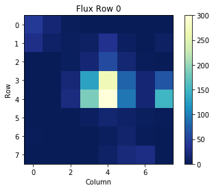
Figure 4: Image centered on the target star, with at least three nearby sources capable of contaminating the sample.
By contrast the photos from the TESS mission, which has much lower spatial resolution but incorporates better data transmission technology, are able to convey all the information collected by its four CCDs back to Earth. A sample of this information can be seen in detail in Figure 5.
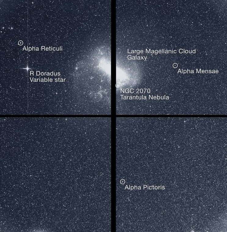
Figure 5: Single CCD image from the TESS space telescope showing the Large Magellanic Cloud and the thousands of stars surrounding it.
The technical difference between the two telescopes makes the observing strategy (taking pictures) completely different. While the original Kepler mission focuses on observing a single corner of the sky, and its extended K2 mission on certain regions of the plane of the ecliptic, the TESS space mission still continues to observe half of the celestial vault each year. See Figure 6.
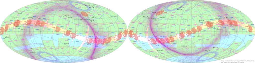
Figure 6: Map of the celestial vault. The field of view of the Kepler/K2 space missions is drawn in orange. The field of view of the TESS space mission is shown in green.
The Kepler/K2 mission focused on small regions of the sky, taking small image snippets of almost a million stars, while the TESS mission is able to take pictures of almost the entire sky (with countless stars) and send the entire picture to Earth.
Once a summary of each of the missions has been given, the scientific community has the challenge of finding the best way to obtain the valuable information stored in each of the photos. So far, the solution has not been especially efficient and consists of extracting the information from those pixels previously defined by a fixed aperture, given a star luminosity previously obtained from the star catalogs.
For the Kepler/K2, normally the star is in the center of the photo cutout, making it more likely that when finding a signal, it will be associated with the main source within the aperture. But the possibility exists that the signal detected in the source is contaminated by a background or nearby star, intense enough to introduce its signal into the selected aperture. In addition, the target star has been previously selected as having a sufficiently high relative magnitude so that contamination from a background star is minimal.
The solution adopted by NASA for Kepler/K2 was simple: apply a fixed aperture for each star according to its relative magnitude. In 80% to 90% of the cases it is an effective aperture, a simple technique to detect exoplanetary signals.
For the TESS telescope, things change substantially. There are thousands of stars in each of the CCDs, so the selection of each star has to be individual and personal, and having lower spatial resolution than Kepler, it is important that the stars aren’t contaminated from another nearby source with a relevant magnitude.
The solution adopted for the TESS mission depends on the research group analyzing the images. NASA distributes the images without any prior filtering, and when we obtain images taken by the space telescope, we need to “clean” and manipulate to extract quality data. In most research groups, light sources are selected using the aforementioned catalogs of stars and galaxies, and the ones with the highest relative magnitude are chosen.
SURFACE LIGHTNING INTO THE PROBLEM
One of the great disadvantages of performing photometry from space is the lack of monitoring of the components of the measurement system. But what does this mean? We simply do not have physical access to calibrate the instruments, making it difficult to know the degradation of the sensitivity of the pixels of each photo over time, beyond the last measurement taken in the laboratory from Earth.
The conditions of spatial resolution in space telescopes whereby a light source takes up only a few pixels (at most tens of pixels), and the lack of calibration, make both aperture and calibration crucial tasks.
As for calibration, several well-established techniques are in use, but aperture still presents a challenge beyond setting a fixed aperture. There are simply too many light sources to search and no efficient means to study them
This problem pertains to both Kepler/K2 and TESS space missions, the first one being in a state of complete data dropout, and with some potential to continue finding more promising signals. TESS, still in operation, has potential to improve its aperture retrieval and locating of bright sources. Automating pixel picking is important with the following considerations:
- Selecting the sky background. In photos with so few pixels, obtaining a sky background for comparison is important.
- Select and mask other light sources present in the image so that they don’t introduce information into our aperture.
- Discard pixels that are bad columns from nearby light sources that have saturated the CCD and have covered more pixels than expected.
For TESS the problem is more significant since its spatial resolution is even lower, and finding a bright source to obtain a good aperture is unlikely . Also, most sources are either not cataloged or cataloged only in certain restricted parts of the sky, making it difficult to know in advance the nearby sources. And even if they were known, a position is only valid for a period of time, and our time frame of consideration is years. While GAIA is doing a very important job in mitigating this problem, once the mission is over, the problem will reappear.
The difficulties will only ensue. With Kepler, examining 150,000 light curves it is not an easy task for even a person specialized in light curves, with only a slight improvement when divided among several experts. With TESS, the situation is unmanageable–with several million light curves, you would need at least a couple of full-time people sorting all the light curves which has a tremendous margin of error due to the rote nature of the task.
APPLYING AI IN SCIENCE: LEVEL UP!
How could we optimize the search for exoplanets in these types of space missions? We have a few options available.
First, we can combine the problem of the choice of aperture and the univocal localization of light sources and use the image recognition technique which involves:
- Detection of light sources in the image.
- Segmentation of each light source, i.e. the specific identification of the pixels occupied by each source in the image.
The next problem is the classification of the thousands to millions of generated light curves that we will obtain. They are all time series but with different cadence, and have the same type of information that is obtained in different ways.
Traditionally, time series have been studied using auto-regressive predictive models. However, neural networks have experienced a very rapid increase in recent years because of their versatility and accuracy, especially recurrent networks combined with convolutional networks. Implementing these techniques to jointly classify any type of light curve is needed to take the search for exoplanets by the transit method to a higher level.
CONCLUSION
The Transit Method is the most common approach to planet hunting and involves detecting a decrease in star brightness as a planet crosses in front of it. However, this method is not perfect and can be hampered by noise from the star or other sources. Machine Learning can help to overcome some of these issues and improve our ability to detect planets using the Transit Method. We are excited about the potential for Machine Learning to play a role in exoplanet discovery and look forward to seeing its impact on this field in the future.